
Sign-up forms were built for humans in browsers, so how do AI agents programmatically register with services?
Enter auth.md. By exposing a single, machine-readable Markdown file at your service root, AI agents can dynamically discover your OAuth Protected Resource Metadata, parse required scopes, and authenticate seamlessly.
With native support in WorkOS AuthKit, you can now implement this protocol out of the box, giving AI tools a standardized, secure way to log into your application.
Airtable holds embeddings for hundreds of thousands of customer databases, and on any given week, roughly three-quarters of them sit completely idle. This fact, more than any algorithm or vendor choice, decided the architecture behind their semantic search system. The interesting story is not which vector database they picked. It is how one peculiar property of their data forced a specific chain of engineering decisions, each one logical only in light of the one before it.
Airtable is a platform where customers build their own database-like applications, organized into “bases” that often hold hundreds of thousands of rows. Their AI feature, called Omni, lets users ask natural-language questions of their data and get answers back in plain English. A separate feature, linked record recommendations, suggests relationships between rows based on meaning rather than exact text matches. Both features depend on the same underlying capability, which is finding the rows in a base that are semantically relevant to a user’s intent.
This might sound simple until scale enters the picture. When a base has half a million rows, fitting all of them into a single LLM prompt becomes infeasible. The model has limits on how much context it can absorb, and even if those limits did not exist, sending that much data on every query would be slow and expensive. The system has to find the most relevant rows fast, then hand those rows to the LLM as context.
In this article, we will look at how Airtable’s data infrastructure team built its architecture, the challenges they faced, the tradeoffs they accepted, and why the choices they made only make sense once their data is properly understood.
Disclaimer: This post is based on publicly shared details from the Airtable Engineering Team. Please comment if you notice any inaccuracies.
The Airtable team anchored their work around four design priorities:
Queries had to return within 500 milliseconds at the 99th percentile, which means the slowest 1 percent of queries still had to come back within that window. Anything slower would make the AI features feel sluggish.
Writes had to be high-throughput since customer data changes constantly, and embeddings have to keep pace.
The system had to scale horizontally to support millions of independent bases.
Everything had to be self-hosted because customer data privacy required keeping it all inside Airtable-controlled infrastructure.
Beyond those priorities, Airtable’s data has three properties worth flagging early:
Customer bases vary enormously in size, with some holding a handful of rows and others holding hundreds of thousands.
Each base is isolated, meaning one customer’s data must never leak into another customer’s results.
Most bases are idle most of the time, a fact that becomes important in a later section.
Before going further, we need to understand what an embedding is.
An embedding is a list of numbers, typically several hundred or a thousand of them, generated by a neural network. The network is trained so that two pieces of text with similar meanings produce numerically close vectors. An embedding can be thought of as a fingerprint of meaning, where similarity in the numbers reflects similarity in what the text says.
One important practical fact is that embeddings are typically about ten times the size of the original data they represent, which is why Airtable cannot just store them alongside the source rows in their primary database. A separate system is needed, one designed specifically for storing and searching across these large numerical vectors.
The asynchronous embedding pipeline that generates and updates these vectors as customer data changes is a separate system, which is the database that stores the embeddings and serves queries against them. After evaluating the landscape in late 2024, Airtable selected Milvus as its database. This is because Milvus supported self-hosting, handled multi-tenancy through its partition model, and let them scale ingestion, indexing, and query execution as separate components. Picking Milvus, though, was the easy part. The hard part was figuring out how to organize Airtable’s data inside it.
See the diagram below:
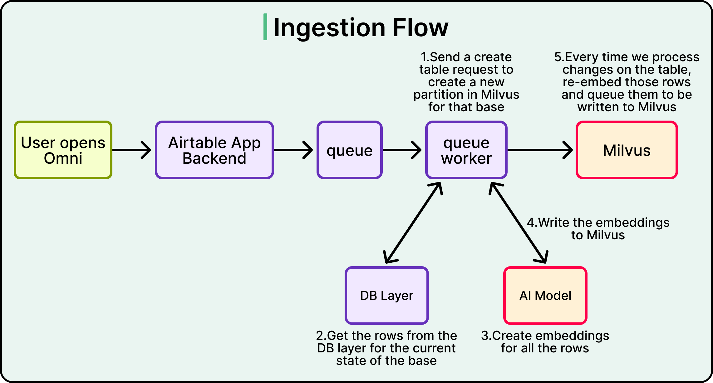
The first real architectural question was how to slice up customer data so that millions of bases can coexist in one system without leaking into each other.
Two options were on the table.
The first option of shared partitions would put many bases together in the same physical slice and rely on a customer ID filter at query time to keep results separate. This approach uses resources efficiently because there is no partition for every customer, and small bases do not sit around taking up dedicated storage. The cost is that every query carries the overhead of filtering by customer ID, and deleting a customer’s data becomes complicated because the rows are scattered across shared partitions.
The second option of having one partition per base gives each customer their own physical slice. Queries are naturally isolated because they only ever touch one partition. Deletion is trivial since dropping the partition is enough. The cost is operational. With millions of customers, the database ends up managing millions of partitions, which puts pressure on its internal bookkeeping.
Airtable picked the second option. The reasoning was that strong physical isolation made permission boundaries obvious, deletion stayed simple, and queries avoided the latency cost of post-query filtering.
Then the team ran into a problem.
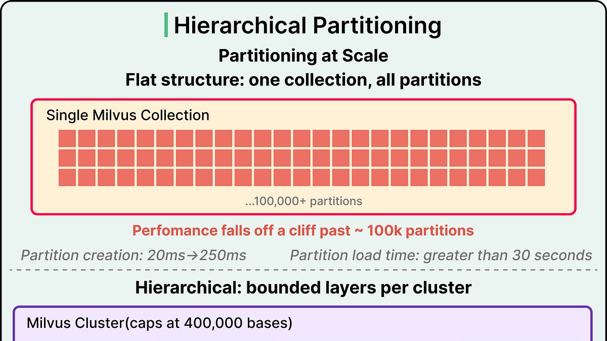
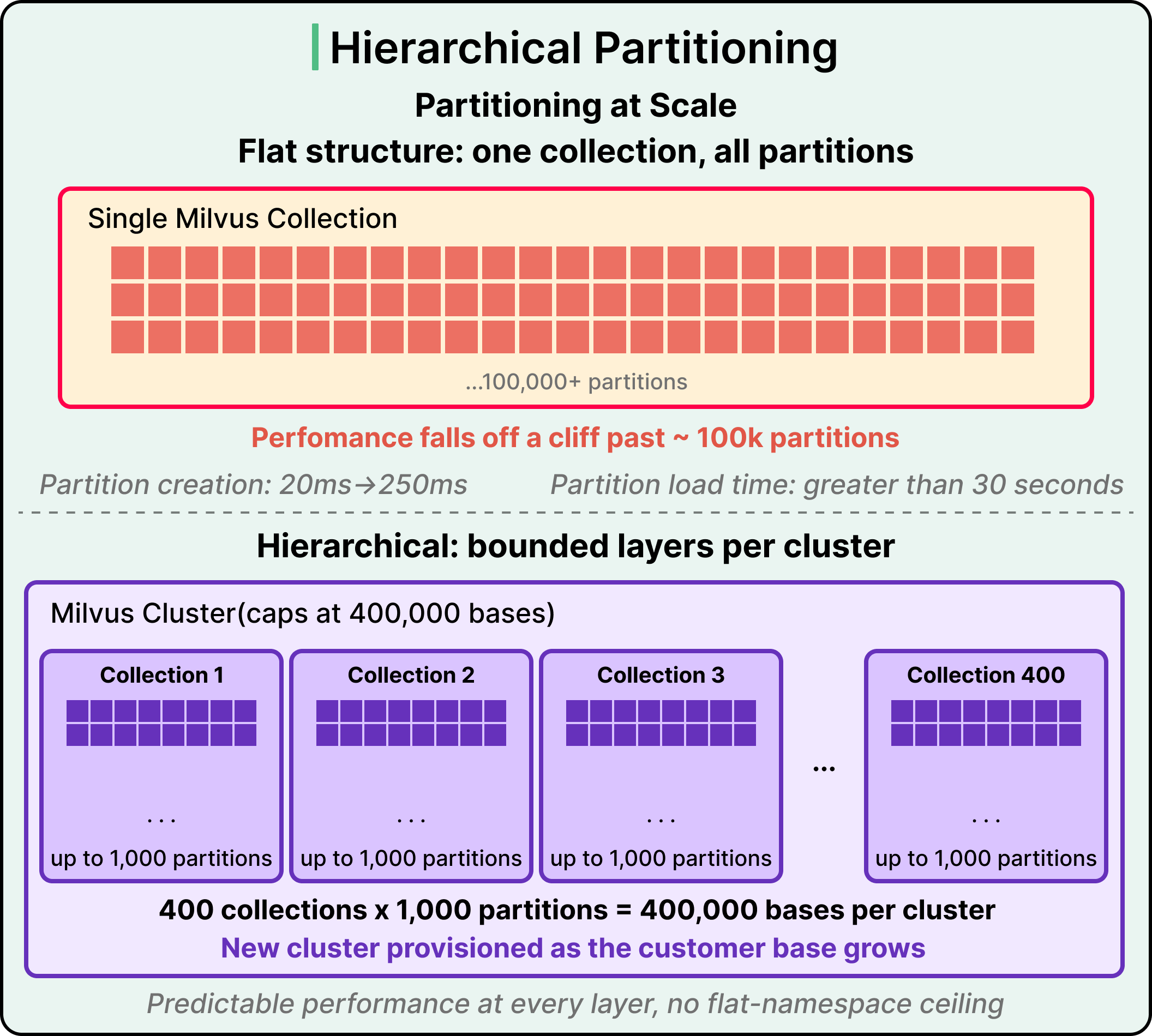
At around 100,000 partitions inside a single Milvus collection, performance fell off a cliff. Partition creation latency went from about 20 milliseconds to roughly 250 milliseconds. Loading a partition started taking more than 30 seconds. Adding hardware would not have fixed any of this, because the issue was not a shortage of capacity. The issue was that too many partitions in one collection overwhelmed the bookkeeping that the database needed to keep them organized.
The fix was hierarchical capping.
Each Milvus cluster now holds 400 collections, and each collection holds at most 1,000 partitions, which limits any single cluster to 400,000 bases. As the customer base grows, Airtable provisions new clusters rather than packing more partitions into existing ones.
The structure trades some operational complexity for predictable performance at every layer. See the diagram below:
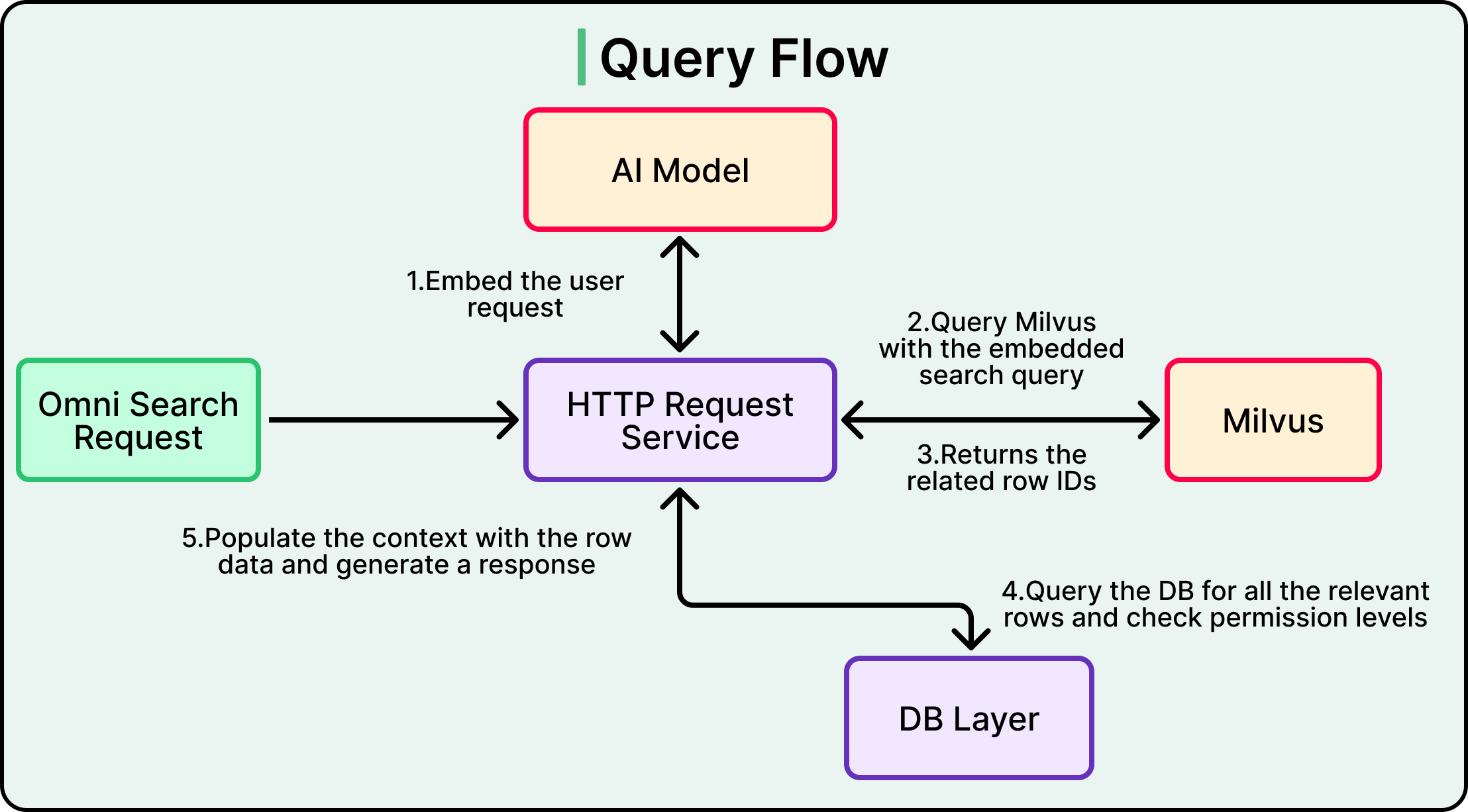
Permissions deserve a brief discussion before we move further. Milvus does not know anything about who is allowed to see what data. It just stores embeddings and returns matches. Permission checks happen later, when the application layer takes the row IDs returned by Milvus and fetches the actual rows from Airtable’s primary database. This split keeps the vector search system focused on a single job, which is similarity search, and authorization stays where authorization always has lived.
The pattern of hierarchical capping shows up across distributed systems, from sharded relational databases to message broker topics. Any flat namespace eventually hits a wall, and the fix is almost always to introduce another level of grouping above it. Recognizing this principle is more transferable than memorizing the specific numbers.
See the diagram below that shows the query flow:
Once the data has been sliced up, the next question is how to actually search inside each slice.
Vector search at scale involves an unavoidable tradeoff with three currencies, namely memory, latency, and recall.
Recall means the percentage of truly relevant results that show up in a query response. Every vector index pays for performance with one of these three currencies, and no option gets all three for free.
Airtable benchmarked three index types, and the results map cleanly onto this triangle.
HNSW, which stands for Hierarchical Navigable Small World, builds a graph where similar vectors are connected to each other. A query starts at a small set of entry points near the top of the graph and follows the connections downward, hopping from one vector to its nearest neighbors until it converges on the closest match. HNSW is fast at lookup time, achieves recall in the 99 to 100 percent range, and behaves predictably under load. The cost is that the entire graph has to live in memory, which makes HNSW the most memory-hungry of the three options.
IVF-SQ8 takes a different approach. The IVF part clusters vectors into groups, so a query only has to search inside the most relevant group rather than the full dataset. The SQ8 part compresses each number in the vector from four bytes to one byte, shrinking the index dramatically. The footprint becomes much smaller, but the compression introduces approximation error that lowers recall.
DiskANN keeps most of the index on solid-state storage rather than in memory. It scales to enormous datasets per node because holding everything in RAM is not required. The cost is that every query touches disk, and disk is slower than memory, so query latency rises.
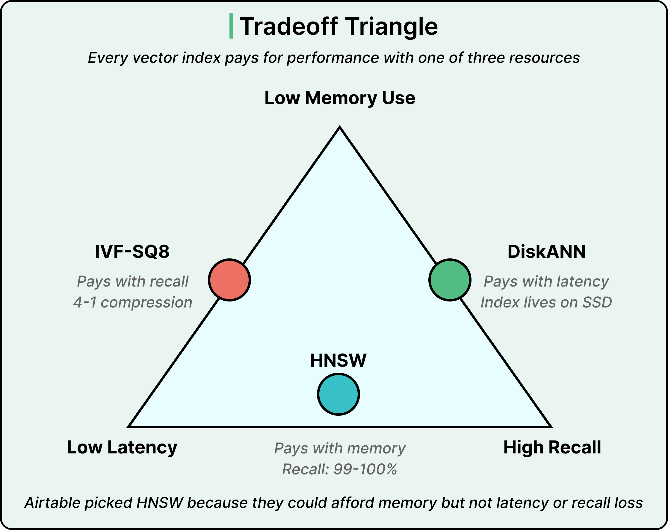
Airtable chose HNSW. Given the priorities from earlier in the design, this was almost the only available answer. A 500-millisecond latency target ruled out DiskANN’s higher per-query cost. The recall directly determines how good Omni’s responses feel to users, which makes the precision of HNSW worth paying for. The memory cost remained a real concern, but Airtable had a separate way to handle it.
The right index does not exist in the abstract. It exists relative to the priorities and constraints of a specific system. If Airtable’s latency tolerance had been looser, DiskANN would have been an interesting candidate. If their recall tolerance had been lower, IVF-SQ8 would have saved them money. None of the three options is universally better than the others.
This same triangular pattern repeats across systems engineering. Caching works the same way, where hit rate trades against memory and consistency. Database indexes work the same way, where read speed trades against write speed and storage. The technologies stop feeling intimidating once the underlying tradeoff becomes recognizable.
Picking HNSW solved the latency and recall problem, but pushed the entire cost onto memory. Across hundreds of thousands of bases, that memory bill adds up quickly. The team needed a way to shrink it without giving up the index they had just chosen.
The solution came from looking at how customers actually use Airtable. When the team analyzed access patterns, they found that only about 25 percent of bases were read from or written to in any given week. The other 75 percent sat completely idle. This was not an anomaly. It reflected something real about how people work. Users tend to focus intensively on one base for a stretch of time, set it aside for weeks or months, and then come back when the project requires their attention again.
Milvus supports offloading partitions from memory to storage and reloading them within seconds. With that capability, Airtable could keep only the hot partitions in memory and push the cold ones out. When a user opens a base that has not been touched in weeks, the partition reloads quickly enough that the user notices a brief warm-up rather than a failure.
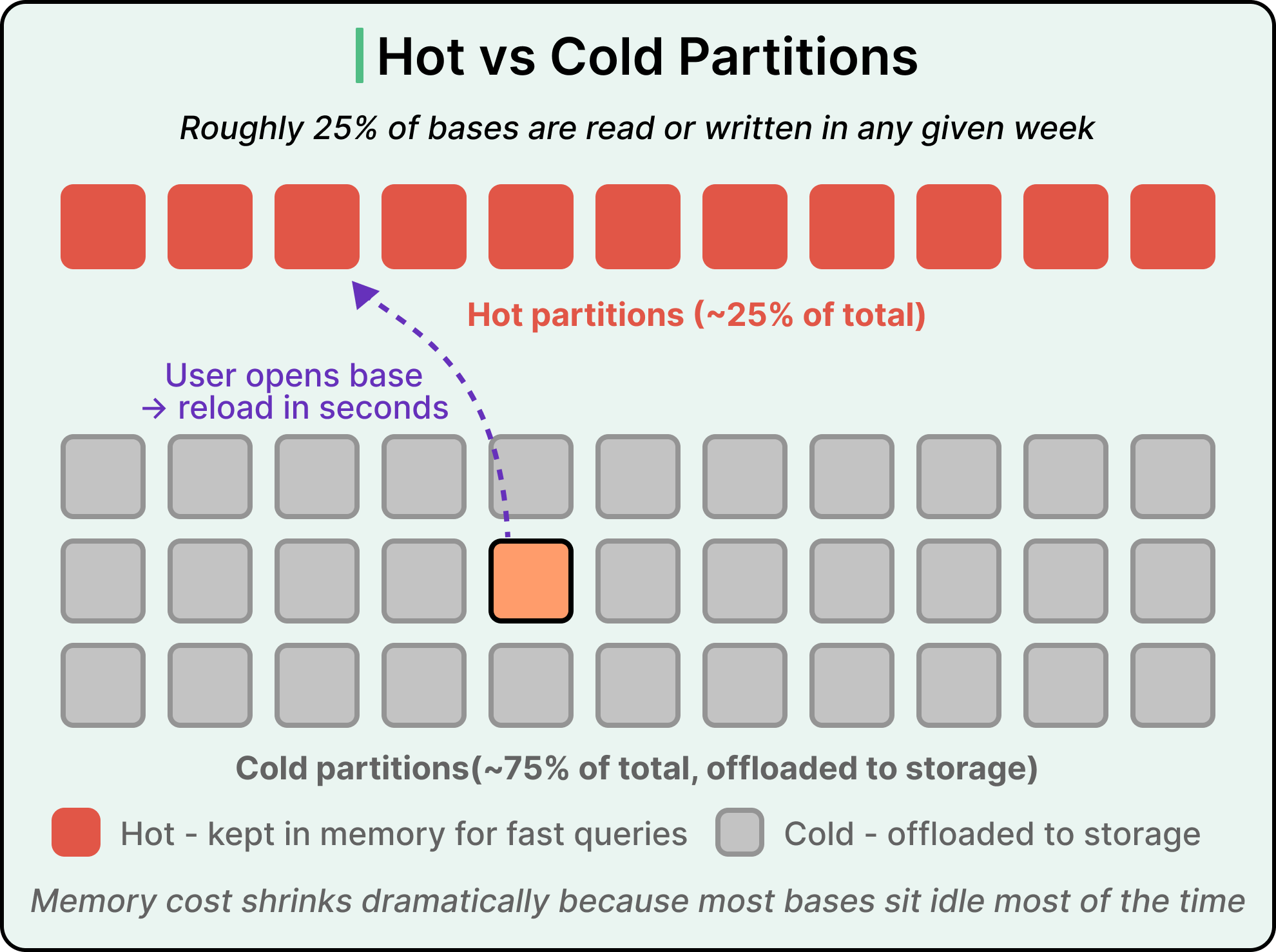
This approach works for Airtable specifically because their access pattern is bursty and bimodal. If usage were spread evenly across all bases, with every customer constantly touching their data at the same low rate, cold offloading would not save much. The hot set would be the entire dataset. Airtable’s pattern is the opposite. A small fraction of bases is active at any moment, and the active set rotates over time.
What made this work was measurement.
The Airtable engineering team did not guess about access patterns and did not reach for a generic optimization. They looked at the data, found a property of their actual usage, and built around it. The HNSW choice became economically viable because of this measurement, and the decisions in this system reinforce each other in a way that would not be obvious from evaluating any one of them in isolation.
The traditional approach to disaster recovery in databases is backup and restore. Snapshots get taken regularly, stored somewhere safe, and used to rebuild the system if something catastrophic happens. Airtable went a different direction.
Their recovery path is to spin up a fresh Milvus cluster and re-embed customer data from the source. The most-used bases get re-embedded first so that most users see normal service quickly. The remaining bases get rebuilt lazily as customers access them. There is some compute cost during recovery and some delay before every base is fully back, but the path is conceptually simple and works across many failure modes at once. Corruption, model migrations, and certain data residency changes all reduce to the same procedure.
This option is only available because Airtable has already built an asynchronous embedding pipeline as part of earlier work. That pipeline normally generates new embeddings whenever customer data changes, processing them in the background rather than blocking writes. Recovery is not a separate system created for emergencies. It is just the existing pipeline running against an empty cluster.
The system built by Airtable involves four major tradeoffs: how to partition the data, which index to use, when to keep data in memory, and how to recover from failure.
Every one of those decisions traces back to the same upstream fact about Airtable’s tenants. Their customers run small, isolated bases that are mostly cold most of the time. Changing any one of those properties can cause the design to fall apart.
For example, a workload where every base is hot all the time would make cold offloading useless. A workload requiring strict consistency would not tolerate the asynchronous embedding pipeline. A workload with very small per-customer datasets might benefit more from shared partitions than from one-per-base.
The technologies Airtable uses, including Milvus, HNSW, and the rest, are interchangeable in principle. The same system could be rebuilt on a different infrastructure, and the architectural reasoning would still hold. What is harder to replicate is the discipline of letting the data drive the architecture rather than the other way around.
References:
[ad_2]
Source link
More on how airtable built the search layer
Stay tuned for updates on how airtable built the search layer as the story develops. Related: Mobile & Accessories.
Frequently Asked Questions
Omni, which answers natural-language questions about data in plain English, and linked record recommendations that suggest relationships between rows based on meaning.
Customer bases can hold half a million rows — infeasible for context limits, and slow and expensive to send on every query.
Queries under 500 milliseconds at the 99th percentile, high-throughput writes, horizontal scaling across millions of bases, and full self-hosting for customer data privacy.
Bases vary enormously in size, each customer's base is isolated from others, and roughly three-quarters of bases sit completely idle in any given week.